Bioinformatics&Statistics
Monday, July 1, 2013
Sunday, June 30, 2013
R Computing
R for bioinformatics
Essential facts
R is a powerful and useful statistical software.
R can be downloaded from the internet free.
For many people, R is difficult and frustrating to learn. but the efforts will pay off in the long run.
The graphics are very basic, and not as impressive or professional looking as SPSS output.
I think that the help menu and features are very useful, poignant, and effective.
You cannot learn very much by reading about R. You must spend quality
time practicing, experimenting, and making frustrating mistakes. The language is
rather cryptic and case-sensitive, which causes silly mistakes, sometimes.
R developers are upgrading R at a seemingly fast rate.
As with most object-oriented programming languages, you end up building a very effective and useful library of small to medium programs, subroutines,functions, and other scripts. All of these R scripts can be linked together into a connected routine, which does complicated tasks quickly and correctly.
Learning R is a valuable exercise in logical thinking, problem solving skills buildup, and fundamental current programming experience
------------
R contains most arithmetic functions like mean, median, sum, sqrt, length, log. Many R functions and datasets are stored in separate packages, which are only available after loading them into an R session
library(my_package) # Loads a particular package.
library(help=mypackage) # Lists all functions/objects of a library.
search() # Lists which packages are currently loaded.
Information and management of objects
ls() or objects() # Lists R objects created during session, they are stored in file '.RData' when exiting R and the workspace is saved.
rm(my_object1, my_object2, ...) # Removes objects.
rm(list = ls()) # Removes all objects without warning!
str(object) # Displays object types and structure of an R object.
ls.str(pattern="") # Lists object type info on all objects in a session.
Reading and changing directories
dir() # Reads content of current working directory.
getwd() # Returns current working directory.
setwd("/home/user") # Changes current working directory to the specified directory.
print(ls.str(), max.level=0) # If a session contains very longlistobjects then one can simplify the output with this command. lsf.str(pattern="") # Lists object type info on all functions in a session.
class(object) # Prints the object type. mode(object) # Prints the storage mode of an object.
summary(object) # Generic summary info for all kinds of objects.
attributes(object) # Returns an object's attribute list.
gc() # Causes the garbage collection to take place. This is sometimes useful to clean up memory allocations after deleting large objects.
length(object) # Provides length of object.
.Last.value # Prints the value of the last evaluated expression.
System Commands under Linux
R IN/OUTPUT & BATCH Mode
One can redirect R input and output with '|', '>' and '<' from the Shell command line.
$ R --slave < my_infile > my_outfile # The argument '--slave' makes R run as 'quietly' as possible. This option is intended to support programs which use R to compute results for them. For example, if my_infile contains 'x <- c(1:100); x;' the result for this R expression will be written to 'my_outfile' (or STDOUT).
$ R CMD BATCH [options] my_script.R [outfile] # Sytax for running R programs in BATCH mode from the command-line
Import
read.delim("clipboard", header=T) # Command to copy&paste tables from Excel or other programs into R. If the 'header' argument is set to FALSE, then the first line of the data set will not be used as column titles.
read.delim(pipe("pbpaste")) # Command to copy&paste on Mac OS X systems.
file.show("my_file") # prints content of file to screen, allows scrolling.
scan("my_file") # reads vector/array into vector from file or keyboard.
my_frame <- read.table(file="my_table") # reads in table and assigns it to data frame.
my_frame <- read.table(file="my_table", header=TRUE, sep="\t") # Same as above, but with info on column headers and field separators. If you want to import the data in character mode, then include this argument: colClasses = "character".
Export
write.table(iris, "clipboard", sep="\t", col.names=NA, quote=F) # Command to copy&paste from R into Excel or other programs. It writes the data of an R data frame object into the clipbroard from where it can be pasted into other applications.
zz <- pipe('pbcopy', 'w'); write.table(iris, zz, sep="\t", col.names=NA, quote=F); close(zz) # Command to copy&paste from R into Excel or other programs on Mac OS X systems.
write.table(my_frame, file="my_file", sep="\t", col.names = NA) # Writes data frame to a tab-delimited text file. The argument 'col.names = NA' makes sure that the titles align with columns when row/index names are exported (default).
save(x, file="my_file.txt"); load(file="file.txt") # Commands to save R object to an external file and to read it in again from this file.
HTML(my_frame, file = "my_table.html") # Writes data frame to HTML table. Subsequent exports to the same file will arrange several tables in one HTML document. In order to access this function one needs to load the library 'R2HTML' first. This library is usually not installed by default.
write(x, file="my_file") # Writes matrix data to a file.
sink("My_R_Output") # redirects all subsequent R output to a file 'My_R_Output' without showing it in the R console anymore.
sink() # restores normal R output behavior.
R Objects:Data and Object Types
Data Types:
Numeric data: 1, 2, 3 ex. x <- c(1, 2, 3); x; is.numeric(x); as.character(x) # Creates a numeric vector, checks for the data type and converts it into a character vector.
Character data: "a", "b" , "c" ex. x <- c("1", "2", "3"); x; is.character(x); as.numeric(x) # Creates a character vector, checks for the data type and converts it into a numeric vector.
Complex data: 1, b, 3
Logical data: TRUE, FALSE, TRUE
1:10 < 5 # Returns TRUE where x is < 5.
Object Types
vectors: ordered collection of numeric, character, complex and logicalvalues. factors: special type vectors with grouping information of its components
data frames: two dimensional structures with different data types
matrices: two dimensional structures with data of same type
arrays: multidimensional arrays of vectors
lists: general form of vectors with different types of elements
functions: piece of code
Factors :Factors are vector objects that contain grouping (classification) information of its components. animalf <- factor(animal <- c("dog", "cat", "mouse", "dog", "dog", "cat")) # Creates factor 'animalf' from vector 'animal'.
animalf # Prints out factor 'animalf', this lists first all components and then the different levels (unique entries); alternatively one can print only levels with 'levels(animalf)'.
animalfr <- table(animalf); animalfr # Creates frequency table for levels.Function 'tapply' applies calculation on all members (replicates) of a level.
weight <- c(102, 50, 5, 101, 103, 52) # Creates new vector with weight values for 'animalf' (both need to have same length).
mean <- tapply(weight, animalf, mean) # Applies function (length, mean, median, sum, sterr, etc) to all level values; 'length' provides the number of entries (replicates) in each level.
Function 'cut' divides a numeric vector into size intervals.
y <- 1:200; interval <- cut(y, right=F, breaks=c(1, 2, 6, 11, 21, 51, 101, length(y)+1), labels=c("1","2-5","6-10", "11-20", "21-50", "51-100", ">=101")); table(interval) # Prints the counts for the specified size intervals (beaks) in the numeric vector: 1:200.
plot(interval, ylim=c(0,110), xlab="Intervals", ylab="Count", col="green"); text(labels=as.character(table(interval)), x=seq(0.7, 8, by=1.2), y=as.vector(table(interval))+2) # Plots the size interval counts as bar diagram.
Tuxedo Suite : RNA seq
Tuxedo Suite:
Tophat (alignment to genome)
Cufflinks
(assembling and
counting of genes/transcripts)
Cuffcompare
(compare
gene expression)
Cuffdiff
(differential gene expression testing)
-----------------------------------
Tophat
Purpose: To identify exon-exon junctions
----------------------
Tophat Command
Tophat Options

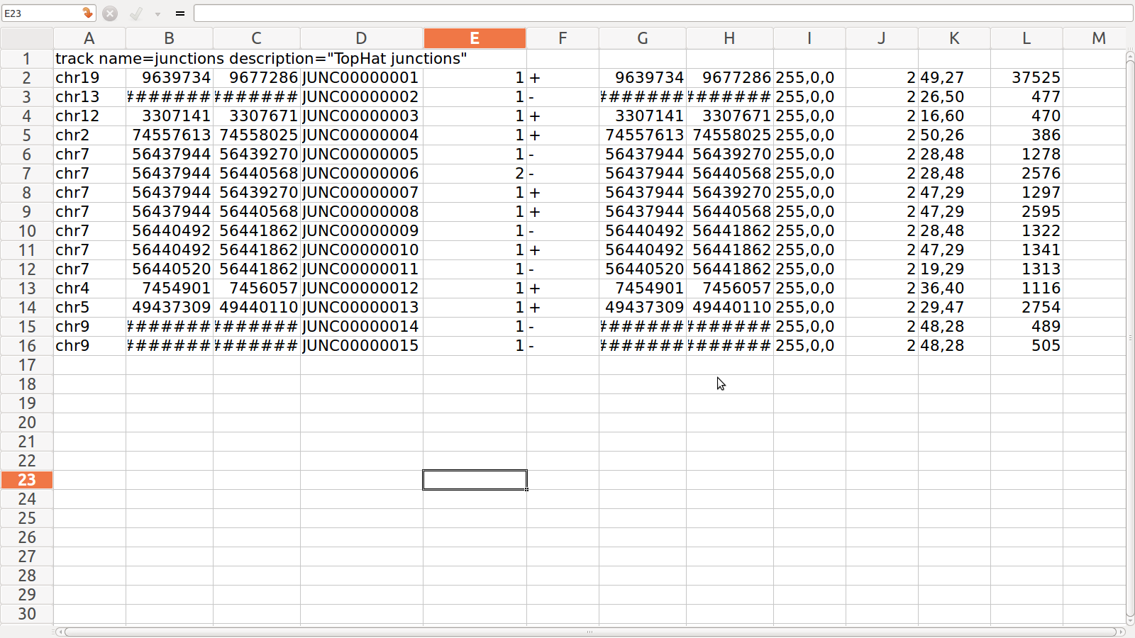
Junction.BED for SRR995

================

SAM Alignment

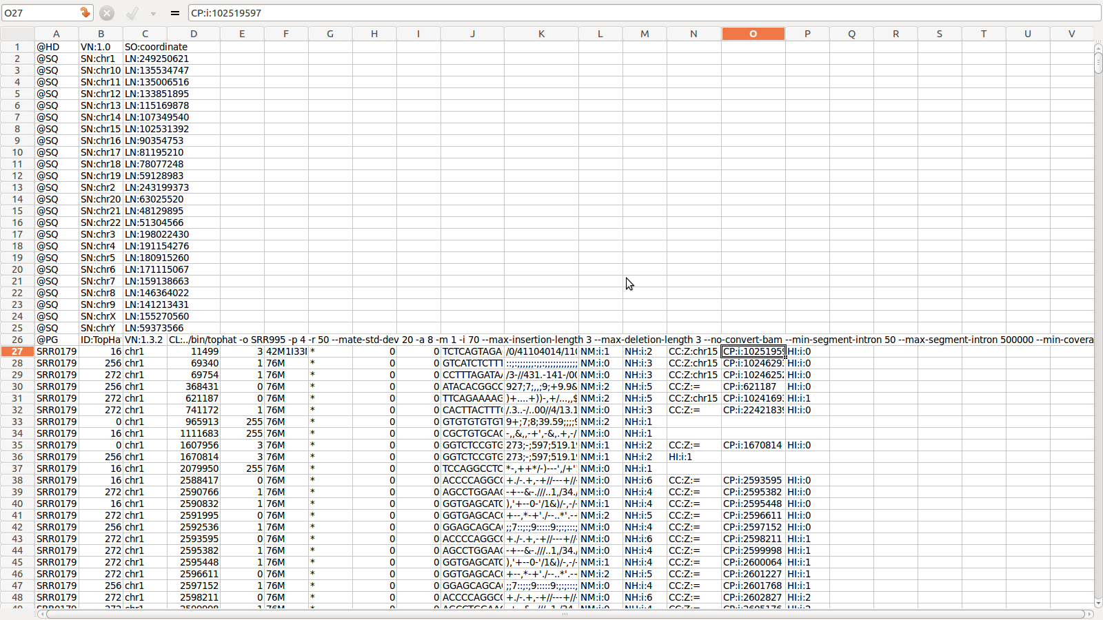
SAM for SRR995

Cufflinks
---Options of Cufflinks
 Secrets of FPKM
-----------------------------------
Tophat
Tophat : maps/aligns RNA seq data to a genome
Note: In order to deal with the problem of splicing in RNA seq data
alignment, you need to use an aligner that is aware of splice junctions
Unique Characteristics: to map
splice junctions de novo, a very handy feature while working on organisms with
incomplete or poorly annotated transcriptomes.(e.g watermelon)
Before Tophat
1. Download species(human)
chromosome file
2. Run the command: > bowtie-build hg19.fa hg19
3. It
will give output index files which should be copied to index folder of bowtie
----------------------
Tophat Command
>../bin/tophat
-o SRR995 -p 6
-r 50 --mate-std-dev 20 -a 8 -m 1 -i 70 --max-insertion-length 3
--max-deletion-length 3 --no-convert-bam --min-segment-intron 50 --max-segment-intron 500000 --min-coverage-intron 50
--max-coverage-intron 20000
--segment-length 25 --keep-tmp --segment-mismatches 2 -I 500000
../hg19 SRR995.fq
•
Note that options are written in red ink
and rest(in blue) are essential.
-----------------------Tophat Options
--output-dir OR -o <filename>: Output location :The default is
"./tophat_out"
--num-threads
OR -p:
number of threads to use
--max-intron-length
OR -i :
Tells tophat to ignore donor/acceptor pairs closer than this many close bases
apart
--min-intron-length
OR -I :
Tells tophat to ignore donor/acceptor pairs farther than this many close bases
apart
-G
<a gtf file>
: tells tophat to use the gtf as a n
annotation reference.
--segment-length
:
each read is cut into this much long segments
-segment-mismatches
:
allows this much mismatches in each segment read alignment
--solexa1.3-quals tells it to use the new illumina
qual values
--keep-tmp: Keep/preserve temporary files
produced during the run.
--no-convert-bam: causes tophat to give SAM file
instead of BAM file
--no-sort-bam: gives output without coordinate
sorting
--min-anchor-length
or -a:
Tells tophat to report junctions spanned by reads with at least this many bases
on each side of the junction.
--splice-mismatches OR -m : max number of mismatches in
the anchor region of a spliced alignment.
--mate-inner-dist
OR -m:
mean distance between mate pairs
--mate-std-dev
O: standard
deviation of distribution of distance between mate pairs.
--no-
discordant :
for paired reads, report only concordant mappings
--max-insertion-length
--max-deletion-length
--segment-length
--min-segment-intron
--max-segment-intron
--min-coverage-intron
--max-coverage-intron
--no-sort-bam
--resume OR -R : tells tophat to
resume in case of failure in the first run
--read-mismatches OR -N : to
ignore those read alignments having more than this much mismatches
--read-gap-length: to ignore
those read alignment having more than this much gap length
--zpacker
OR -z:
to specify that all tmp files are in compressed mode
-z0: to disable compression
---------------------------------------
Tophat Output
1. junction.bed: it lists BED track of junctions
reported by Tophat where each junction consists of two connected BED blocks
where each block is as long as the max overhang of any read spanning junction
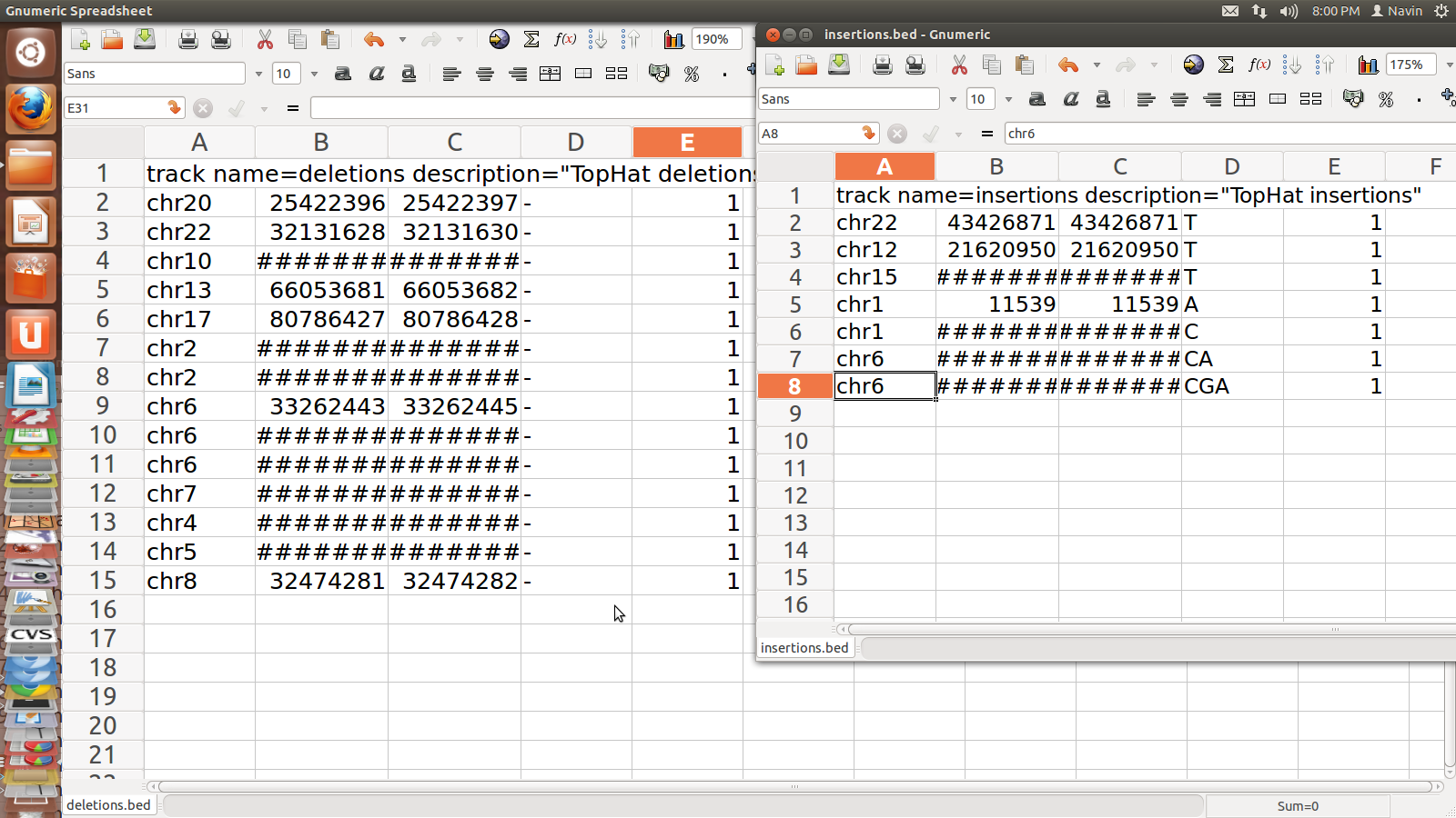
2. deletion.bed: mentions the first genomic base of the
deletion
3. insertion.bed:mentions the last genomic base before
the deletion
4. accepted_hits.bam(/sam):
A
list of read alignments in BAM/SAM format
Let us explore SAM file format in coming
slides
---------------
Insertion.bed
and Deleton.bed for SRR995
Junction.BED for SRR995
================
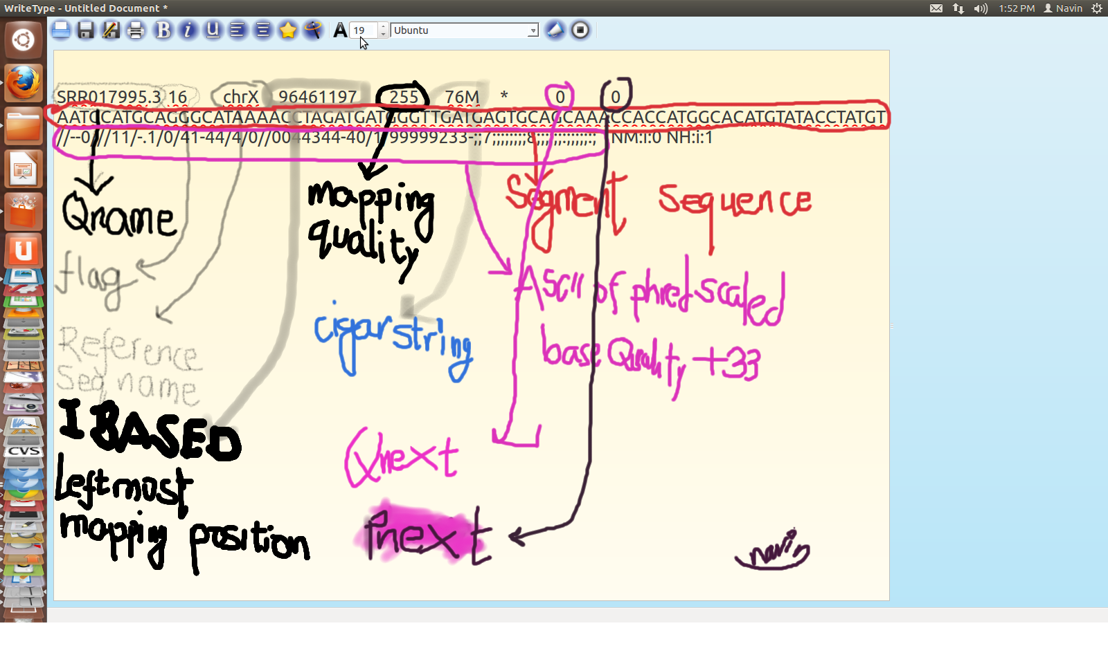
SAM Format
A generic file format for storing large nucleotide sequence alignment in compact manner.
It is marked for
a. flexibility to store alignment from various aligners
b. easy creation from aligners and also convertibility from other other file formats
c. capacity to allow operations on alignment to work on stream without loading whole genomic data
d. allows the file to be indexed on genomic position
Structure of SAM
SAM Alignment
SAM for SRR995
Cufflinks
Cufflinks assembles transcripts, estimates their abundances and tests for differential expression and regulation.
Cufflinks module consists of cufflinks, cuffcompare and cuffdiff (and cuffmerge) commands
It accepts aligned RNA seq read alignment and assembles into a parsimonious set of transcripts
It estimates relative abundances of each transcript. It is based on how many reads support each transcript
---Options of Cufflinks
cufflinks [options]* <alignedreads.bam or .sam>
SAM is a standard short read alignment that allows aligners to attach custom tags to individual alignments and Cufflinks requires that alignments have some of these tags
Option : -g (or -G) species.gtf is a must As this is an annotation file where all genes/transcripts of the species have ids and tags.(Identity Collection)
-G <reference annotation gtf file> : to estimate isoforms abundances but ignore novel ones
-g <reference annotation gtf file> : to estimate isoforms abundances as well as novel ones
- p and -o are have the same meaning as that in tophat.
-M OR --mask-file:Tells cufflinks to ignore those reads which could have come from the specified transcript file
-b OR --frag-bias-correct: frag bias correct : torun bias detection and correction algorithm so as to improve accuracy of transcript abundance estimates
-m OR --frag-len-mean : average fragment length: The default is 200bp
-s OR --frag-len-std-dev : standard deviation of distribution of fragment length : Default is 80bp.
-N OR --upper-quartile-norm : normalized by upper quartile to improve robustness of differential expression calls for less abundant genes and transcripts
Note: Cufflinks now learns the mean and std dev of fragment length for each SAM file so using options -m and -s is no longer recommended
--total-hits-norm: to count all fragments
--compatible-hits-norm: to count fragments comptible with reference annotation
--max-mle-iterations : to set number of iterations allowed during max likelihood estimation of abundances
-p , -o, -G have same meaning as that in Tophat options
Cufflinks Output
1. transcripts.gtf
Column number
|
Column Name
|
Example
|
Description
|
1
|
seqname
|
chr
|
chromosome name
|
2
|
source
|
cufflinks
|
program which generated
|
3
|
feature
|
exon
|
type of record: either transcript or exon
|
4
|
start
|
455666002
|
leftmost coordinate of this record
|
5
|
end
|
455666978
|
rightmost coordinate of this record
|
6
|
score
|
455666978
|
strnd from which the isoform came from
|
7
|
strand
|
+/-
| |
8
|
frame
|
.
| |
9
|
attributes
|
see the next page
|
Attributions of GTF file
1.gene_id
2.transcript_id
3. FPKM
4. frac
5. conf_lo: Lower bound of the 95% confidence interval of the abundance of this isoform, as a fraction of the isoform abundance is determined from this number
6.conf_hi: Upperbound of the 95% confidence interval of the abundance of this isoform, as a fraction of the isoform abundance is determined from this number
7. cov: Estimate for the absolute depth of read coverage across the whole transcript
8. full_read_support
2. isoform.fpkm_tracking: This file contains estimated isoform level expression levels in FPKM tracking format
3. genes.fpkm_tracking: This file contains estimated gene level expression levels in FPKM tracking format
-------
Glimpse of one row of gtf file
- FPKM : a measurement of pair of transcript reads that has been normalized both for transcript length and for the total number of mappable reads from an experiment.
- This normalized number helps in the comparison of transcript levels both within and between samples.
-------
Cuffcompare
It takes Cufflinks GTF output as input and optionally can take a reference annotation and gives 5 output files including combined.gtf which contains union of all transflags. If a transflag is present in both samples, it is thus reported once in the combined gtf.
It helps analyze the transflags we assemble
It compares the assembled transcripts to the reference annotation
It tracks cufflinks transcripts across different experiments.
Run the command as
cuffcompare [options]* cuff1.gtf cuff2.gtf cuff3.gtf
where cuff?.gtf are outputs of cufflinks
Cuffcompare Options
-r : An optional annotation reference file. Each sample is matched against this file and sample isoforms are tagged overlapping or matching or novel one depending on case.
-R : it tells the cuffcompare to ignore those reference transcripts which are not overlapped by any transcript of any sample gtf
-s : causes cuffcompare to look into fasta files with the underlying genomic sequences against which your reads were aligned for some optional classification function.
-V: verbose: it will write what cuffcompare is doing and also showing any warning
-o: Directory of output file :
-r :tells it to use annotation.
-R ; tells it to leave out transcripts not present in any sample
-s: switch for some reason is necessary to propagate the gene names through to the next step properly.
Subscribe to:
Posts (Atom)